Time and Space Complexity in DSA
-
Time and Space Complexity is an important measure of how well an algorithm performs for a particular type of data structure and depending on the number of input values. In general, as the number of input values increases, time taken to complete the process and also the memory needed increases.
Time and Space Complexities can be measured in terms of best, average and worst case scenario. It is better to do the calculation based on the worst case scenario to identify better performing algorithms.
For example, while doing a Sequential search for a particular number from an array of numbers;
- Best case scenario is that the number located at the first position. Just one iteration is needed.
- Average case scenarios are the most occurring ones, where the number resides more to the middle of the array.
- Worst case is that the searched number is located at the end of the array.
Time and Space Complexities of an algorithm is expressed in terms of Big O notation
Big O notation
Time and Space Complexities of an algorithm is expressed in terms of Big O notation. Big O notation represents functions according to their growth rates.
In Big O notation, space and time complexities are represented like O(n). Letter 'n' represents the size of the total number of bits needed to represent the inputs.
-
Time complexity
Time Complexity represents the the amount of time required to complete an algorithm run for a given number of inputs.
Most of the algorithms that perform a particular data structure operation will be required to do some tasks repeatedly until the final output is reached. Time complexity is generally measured by counting the number of these iterations required to complete the task for a worst case scenario.
Also keep in mind that, here we are assuming that each iteration is going to take exactly same amount of time. But in real scenarios slight variations can be there and we are not considering that.
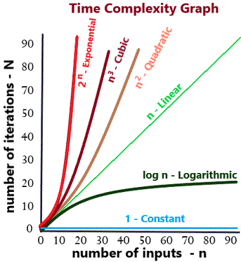
The line that starts from (0, 0) and propagates diagonally to the top-right corner represents linear time complexity. Ideally the best performing algorithms are expected to be of complexity below linear time complexity, although some of the most used algorithms like Bubble Sort run above this line.
Let us understand what each of these mean.
-
Constant Time Complexity
Represented as O(1). Note that, here 'n' is not mentioned in the notation. That means number of inputs is not relevant here. And only one iteration is enough to find the output. Many of the code that we write are of this category.
As an example, consider finding the length of an array. No matter how much is the number of inputs, last index - 1 is always the length and only one iteration is enough for this.
-
Logarithmic Time Complexity
Represented as O(log n). Logarithmic time complexity algorithms can be considered as the best performing algorithms that does a repetitive task. This always performs better than algorithms of linear complexity.
These types of algorithms tend to perform better for higher input numbers. Examples include searching from a sorted array, binary tree search, etc. For each iterations, these algorithms eliminate the remaining half of the input entries and gets the output fast.
-
Linear Time Complexity
Time complexities explained above are known as Sub-linear time complexities and and are considered best performing. Linear Time Complexity is represented as O(n). These type of algorithms require exactly the same number of iterations as the input numbers.
Example: Finding the sum of all elements in an array.
-
Quadratic, Cubic and Polynomial Time Complexities
- Quadratic - O(n2)
- Cubic - O(n3)
- Polynomial - O(poly(n))
Quadratic time complexity algorithms take iterations to the square of the input numbers. Generally needed for algorithms like Bubble Sort that requires a loop to run within another loop. Similarly for cubic time, three nested loops are required.
For a Polynomial time, n, is calculated as the output of a Polynomial equation.
-
Exponential Time Complexities
Exponential Time Complexity is represented as O(2poly(n)). These type of algorithms tends to be an inverse of Logarithmic Time Complexity algorithms. Iterations increase exponentially to the number of inputs.
Brute force search algorithms come under this group. An example is finding all the possible paths in a map. From each node of the map, we can turn to all the connected nodes and each of these creates a new path.
-
-
Space complexity
Space Complexity represents the the amount of memory space required to complete an algorithm run for a given number of inputs. This is also represented using Big O notation.
Different types of complexities explained for Time exists for Space as well. But we cannot measure Space complexity in the same way as of Time simply because the repetitive processes in some algorithms can use the same memory location for each iteration and in case of some algorithms this may not be possible.
The algorithms that perform best in case of time complexity tend to use more space and vice versa. For example, a sequential search is a slow process, but doesn't require any additional memory to store temp data. But in case of divide and conquer algorithms that perform better in terms of speed needs to store temporary data in queues or stacks and consumes more space.
Also keep in mind that the space complexity varies depending on the programming language used, as the memory allocation process has differences among different languages.