Array Data Structure
-
We know that an Array Data Structure or simply Array is used to store a collection of data of similar types. Each item in the array can be considered as a node. Nodes can be of any primitive data type like, integer, string, char, bool, etc. Each node can even be another array. Such configuration is known as two-dimensional array.
Arrays usually hold data of same type. This is because at the time of declaring the array we need to specify the limit. And as per the limit size, total memory is allocated for an array in advance.
Suppose we are creating an array of size 10 of Integer data type. In most programming languages 4 bytes are allocated for each Integer type variables. So for an Integer array, a total of 40 bytes should be enough if size is 10.
Now if we want to insert a number of Double data type to this array, it will not work. Because to represent a double data type more bytes are needed (usually 8). There are work-arounds like creating array of Object data type, but will result in unwanted memory usage and is better to avoid.
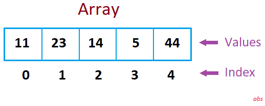
Arrays can be accessed using the index values, which are essentially number sequences that start with 0 or 1. Most languages use zero-based indexing (starting with 0).
-
Dimension of an Array
As mentioned, arrays can hold primitive data types or an another set of arrays. When arrays are stored within another array, it becomes multi-dimensional. Arrays can extend to any dimension.
Let us check some samples.
Single-dimensional
Declaration : int[] ar = new int[10];
Data Representation : [10, 4, 7, 9, 15, 29, 20, 30, 11, 5]
Data Access : var i5 = ar[4] Ans: 15Two-dimensional
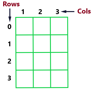
Declaration : int[][] ar = new int[4][3];
Data Representation : [ [10, 4, 7, 9], [15, 3, 2, 1], [4, 11, 9, 8] ]
Data Access : var r2c3 = ar[1, 2] Ans: 3Three-dimensional
Declaration : int[][][] ar = new int[3][2][2];
Data Representation : [ [[1,2], [4,5], [7,8]], [[1,2], [4,5], [7,8]] ]
Data Access : var x2y2z1 = ar[1, 1, 0] Ans: 4As you can see, dimension is the number of indices required to access an element. Multi-dimensional arrays are useful in representing matrices, vectors, graphs, diagrams, maps, etc.
-
Variable Length Arrays
Some languages allow creation of variable length arrays. In a two-dimensional array we need to specify the number of rows and columns. Declaring an array int[][] ar = new int[4][3], creates a matrix structure of 4 rows and 3 columns as below.
For variable length arrays, number of columns for each row varies. This needs to be declared as below. Make sure to declare all column length before using the array.
int[][] ar = new int[4][];
ar[0] = new int[3];
ar[1] = new int[2];
ar[2] = new int[4];
ar[3] = new int[1];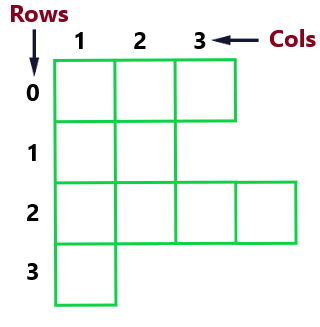
-
Array Sort
An array data structure is said to be Sorted, if its contents are arranged in ascending or descending order of numbers, alphabets or any other data. Sorted arrays helps in faster search by using Divide and Conquer algorithms.
Some of the most commonly used sorting algorithms are below. Click on the links to get more detailed explanations and sample code implementations.
-
Merge Sort
Merge Sort is an algorithm that follows Divide and Conquer method, making it fast and efficient and is useful in many scenarios.
Merge Sort splits the array into n number of sub-arrays (n is the length of the array). Then each item is merged back, in-order to get the sorted array.
Time complexity of Merge Sort is O(n log n).
-
Heap Sort
Heap Sort is an improved version of selection sort. It divides array into sorted and unsorted sub-arrays. Then it fetches the largest or smallest element from unsorted arrays and inserts into the sorted ones and then combine all sorted arrays.
Time complexity of Heap Sort is O(n log n) for all scenarios.
-
Quick Sort
Quick Sort is also a Divide and Conquer algorithm. This works by splitting arrays to two based on a pivot element and then doing the recursive sorting of sub-arrays.
Quick Sort performs better than Merge and Heap Sort in some cases. But if not well defined, it can fail and can take long time to complete. Worst case scenario time complexity is O(n2). Average performance is of the complexity O(n log n) which is almost same as merge sort.
-
Bubble Sort
Bubble Sort is an algorithm that iterates through the array and compare adjacent nodes and re-arranges it. This process repeats n number of times, where n is the length of the array.
Performance wise Bubble Sort is bad and is rarely used in real world scenarios. But the logic is simpler and easy to understand, making it useful for beginners to start with DSA concepts. Time complexity of Bubble Sort is O(n2).
-
Selection Sort
Selection Sort is an in-place comparison algorithm. Its performance complexity is O(n2), similar to Bubble Sort, which makes it in-efficient and is not usable in cases where data is large.
-
Insertion Sort
Insertion Sort is also a low performance algorithm with complexity O(n2) on average. However, it tend to perform better compared to other sorting algorithms of similar complexity.
-
-
Array Search
Searching is one of the most important and and most performed operations on a data structure. Searching is the process of navigating through a data structure and finding all matching items.
To search an array we can use algorithms like;
-
Linear Search
Linear Search is a sequential process of finding an item within an array using a loop.
Linear Search is rarely used for practical cases, because there are other algorithms of logarithmic complexity that uses Divide and Conquer methods to find results much faster.
Time complexity of Linear Search is O(n) for worst case and O(n/2) for average.
-
Binary Search
Binary Search is performed on a sorted array. This basically compares the search element with the middle element of the remaining array. Then checks if it is greater or lesser or equal and eliminating the other half for each iteration, till the result is obtained. Binary search is a well performing algorithm and has many practical applications.
Time complexity of Binary Search is O(log n) and space complexity is O(1).
-
Jump Search
Jump Search is also performed on sorted array. It jumps a predefined interval for each iteration and checks if the search element is greater or lesser or equal to the current node element. Once the searched element becomes bigger than the current node value, it adjusts the interval and moves backward. This process repeats till the result is found.
Jump Search has better performance than Linear Search and is worse than Binary Search.
-
Interpolation Search
Interpolation Search is a variation of Binary Search and is performed on sorted arrays. Simply put, instead of picking the middle position for comparison, a random position is picked continue the search.
-
Exponential Search
Exponential Search is also performed on sorted arrays in 2 stages. First stage identifies a range that can contain the searched item. In second stage, a Binary Search is performed on this range.
Speed depends on how fast the first stage completes. Suitable for certain type of data only.
-
Fibonacci Search
Fibonacci Search is performed on sorted arrays similar to Binary Search. The difference is that Fibonacci Search divides arrays of the size of 2 consecutive Fibonnaci numbers.
For example, for an array of size 8, sub-arrays of size 3 and 5 are created. Fibonacci search uses addition and subtraction instead of division in Binary Search. Although this is of not much relevence now, at the time of its introduction in 1950s, addition and subtraction had significant performance advantage over multiplication and division.
Time complexity of Fibonacci Search is O(log n) similar to Binary Search.
-
-
Array Traversal
Array Traversal is the process of navigating through an array data structure. This can be done to do a sort, a search, finding the sum of few items in the array, etc.
For traversal, we need to implement a loop. See below a sample code snippet in Java to loop through an array and find the sum of all elements.
Copiedint[] ar = { 20, 40, 30, 10, 50}; int sum = 0; for (int i = 0; i < ar.length; i++) { sum += ar[i]; } System.out.println(sum); -
Array Insert/Update/Delete
Array Insert, Update or Delete operations manipulates the contents of the array. Most of the programming languages provides built-in methods to manipulate the array data and is easy to implement. Although, behind the scenes, array traversals and searches are happening.